Reconstructing animal movements in 3D naturalistic environments from field measurements

Rats are highly intelligent social creatures who co-evolved with humans in cities¹. They also damage infrastructure and pose zoonotic and mental health risks to people—and their numbers are rising with global warming and urbanization. Yet we understand surprisingly little about the intelligence of wild animals like rats, since most controlled studies must be done in the lab.

At Basis, we’re working to uncover basic principles of intelligence, while helping mitigate intractable societal challenges. Our collaborative intelligent systems group researches animal social behavior, with a core focus on urban rats. This team has recently been testing and developing new computational tools to study animal behavior in their natural habitats.

To analyze rat behavior in the wild, we need to collect and analyze accurate, high-resolution movement data, embedded in a faithful reconstruction of the outdoor scene. This post describes various tools we have been developing for these tasks, with the deliberate goal of creating a working operational pipeline that is able to process recordings automatically as they are collected, within reasonable computational costs. This automation dream largely dictates our choices of frameworks, tools, and algorithms.

This technical blog post outlines some of our latest techniques for creating ‘world models’ of animals’ natural environments, and characterizing social behavior of animal ‘agents’ within these environments. It is meant for a technical audience. For those less interested in the technical details, we hope you enjoy some of the fun visualizations; see also our rats@basis FAQ page, as well as popular media and news coverage of Basis’s rat project.

Reconstructing the environment

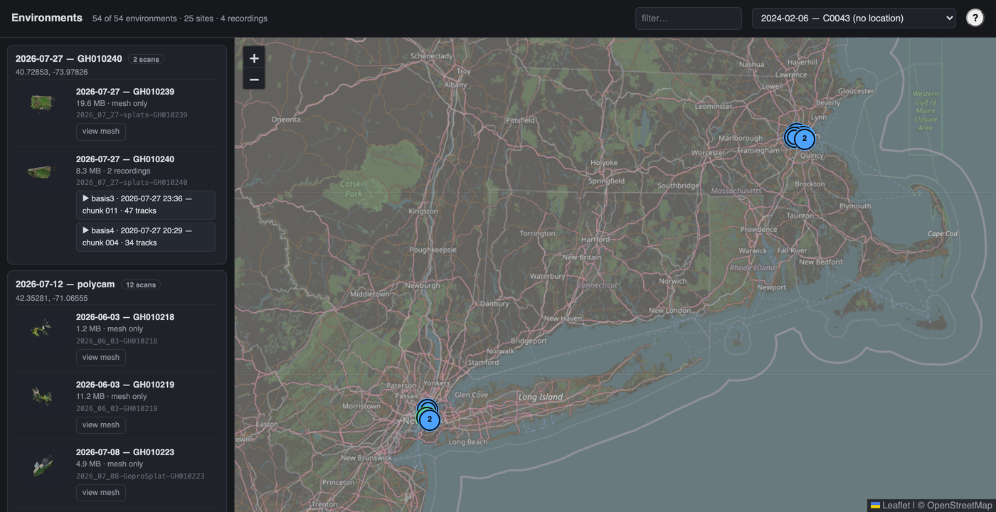
We start by capturing a “walk-through” recording of the site, which is then processed to produce an accurate 3D point cloud or a mesh representation of the scene, preserving high visual fidelity. For the recordings we mainly use GoPro cameras, although we have also had good results using direct depth capture on LiDAR-equipped mobile devices. We have observed that the best quality recordings come from traversing the scene with smooth, continuous motion and capturing all locations from multiple angles (e.g., at multiple heights around a given object). The 3D geometric representation can then be generated by a variety of methods, such as 3D Gaussian Splatting ² or Visual Geometry Grounded Transformer (VGGT) ³, plus a meshing step. The resulting output quality tends to depend on various factors, such as scene complexity and recording conditions. For quick generation, we found the Polycam online platform to work great, and for more customized reconstructions we use our own stack ⁴.

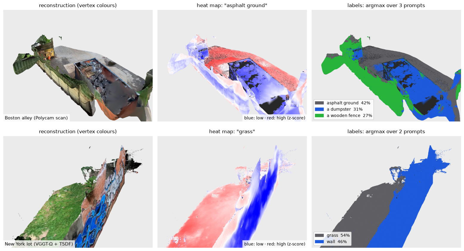
Given that environments were recorded in different locations, we aimed to capture the diversity of information within these environments by extracting semantic information for each 3D point. While many semantic segmentation approaches exist, we chose the particularly appealing Talk2DINO ⁵ approach, where arbitrary text prompts get projected onto a visual feature space, giving each image patch (or, in our case, each mesh vertex) a similarity score. The result is a heatmap for each query, which can then be combined into global label maps by argmax.

Synthetic data generation

In order to improve and test our tracking, we establish a synthetic data generation pipeline capable of producing realistic-looking videos of animals moving within the reconstructed or generated 3D environments. This is standard practice in animal behavior research. ⁶

We base our pipeline on Blender, an open-source 3D computer graphics suite with an excellent Python API. The philosophy of the pipeline is simple: do things that are tedious in code, in the GUI; do things that are tedious in the GUI, in code.

The first step is to create a scene in the GUI. We do this either by dropping in existing assets such as a dumpster model or by importing a scanned real-world environment.

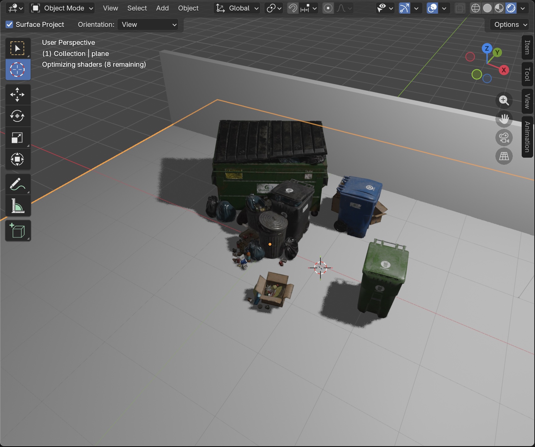
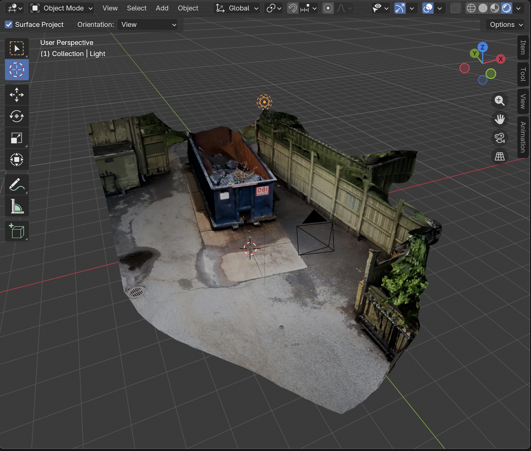
The second step is to populate the scene with rats. For each rat, we specify its movement path by picking 2D points from a top-down view and handing them over to the Python pipeline alongside the Blender file. The height coordinate is automatically inferred for us and the points are connected with a Bézier curve.

In the next step, we specify how each rat should behave along its path. We use a 3D rat model by Nestaeric with a generous usage license. It provides several animations for walking, running, or idling; check them out below:

• each animation plays to completion,

• walking and running animations match the movement speed along the path,

• transition animations between walking, running, and idling are added automatically.

As an alternative to this manual approach, the pipeline also accepts input trajectories from any source and attempts to render them with rat animations.

Finally, we can export the generated data. This includes RGB / thermal-like videos, ground-truth bounding boxes, depth and obstacle maps, as well as the intrinsic coordinates of the rats in the coordinate frame of the surface on which they move. Check out the generated videos below:

Tracking animals in thermal videos

Accurate tracking of populations within their lived 3D environment is essential for the quantitative study of animal behavior. ^{1 4 7} Tracking from video footage relies on accurate detection of the animals in each frame. For nocturnal or camouflaged animals, like urban rats, thermal cameras are essential, but often lead to noisy detections, partly due to relatively coarse spatial resolution of typical recordings. Various additional factors complicate tracking: a varying number of animals per frame, varying animal sizes, multiple animal species, animals “huddling”, erratic movements, occlusions and complex 3D environment geometry.

Our typical setup consists of a single thermal camera mounted on a tripod, recording rat movements for a few minutes each time.

Track in 2D, lift into 3D

While we are working on a direct 3D tracking algorithm that tackles many of the above challenges (see below), in our current production pipeline we take a two-stage approach: track in 2D first, lift into 3D later.

For the first stage, we use a combination of a fine-tuned YOLO ⁸ detection model trained on hand-labeled thermal frames, and a simple blob detector, whose output is then passed to the ByteTrack ⁹ algorithm.

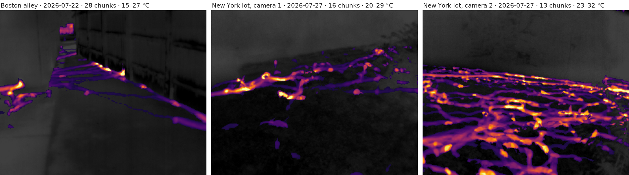
Typically we convert the raw thermal footage into grayscale video. To calibrate the temperature range for the detector, we compute a simple motion/temperature score for each pixel in each frame, resulting in an empirically accurate movement trace across the viewport.

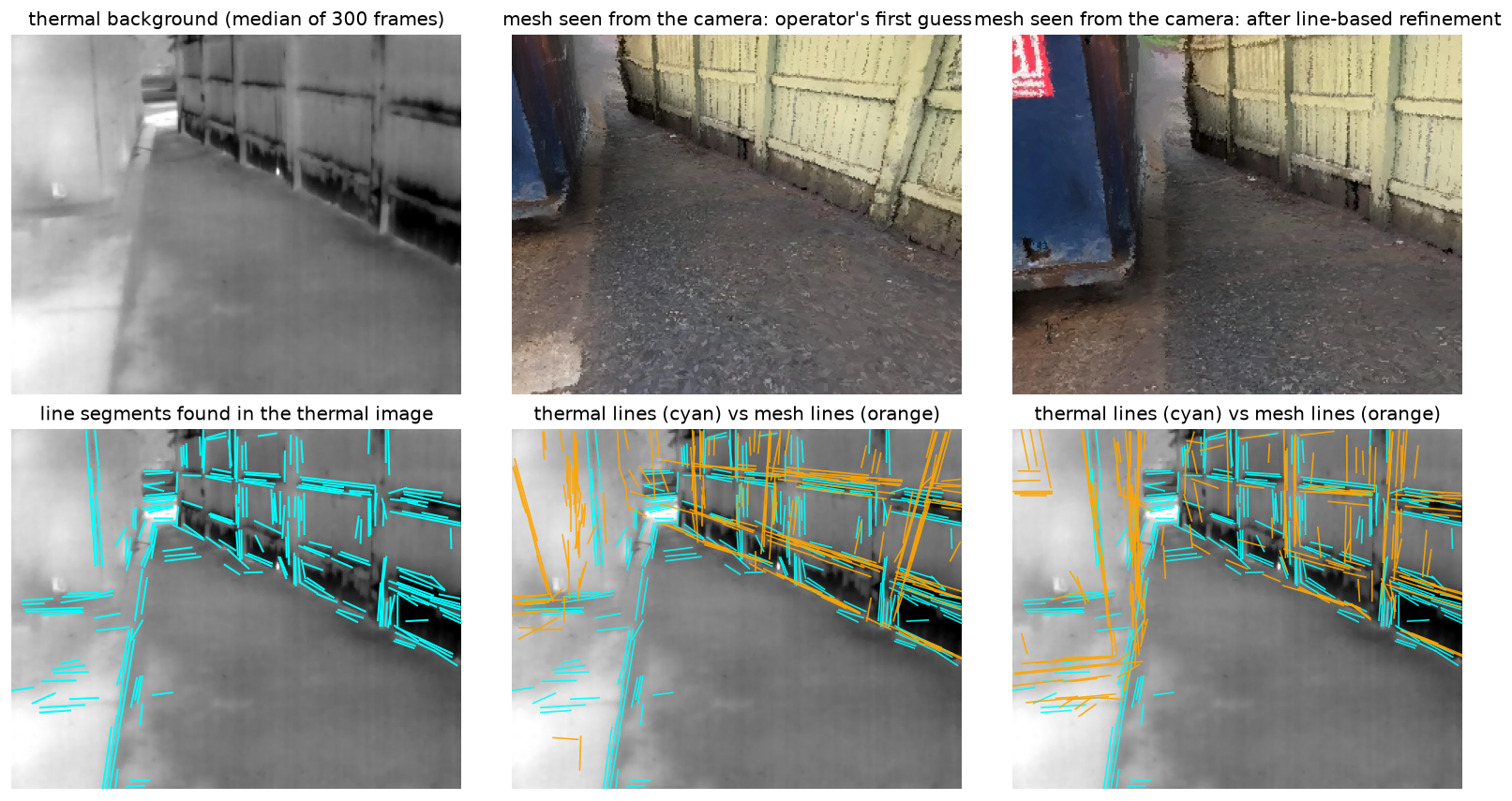
In the second stage, we need to find the actual 3D position of each detected object in each frame. While the most general 2D-to-3D lifting problem is ill-posed for some animals (e.g., birds require an additional source of information such as a simultaneous recording from a second camera), in this work we assume that our animals (wild rats) move on stable surfaces. Consequently, we can use the depth map corresponding to the visible part of the mesh in the global 3D coordinate space, and solve the reprojection problem uniquely. The only remaining task is to find the actual thermal camera pose. If our tracking video is RGB, we can use feature matching in a common visual feature space ⁴. However, this approach is challenging for thermal/RGB matching (although there is some work in this area ¹⁰). As a current workaround, we use a hybrid approach where we start with a manual approximate match of the mesh and thermal view, and optionally fine-tune the camera intrinsics and extrinsics by minimizing an oriented Chamfer distance between the sets of salient edges in the two images.

The robustness of the method can be improved by imposing constraints on the reprojected tracks, and, ultimately, switching to a joint optimization of the 3D camera pose and the tracking output itself.

Particle filter approach to 3D tracking

Everything so far lifts tracks into 3D after tracking them in 2D, so every identity switch and lost track in the image is inherited. To address these issues, we designed a tracker that reasons in 3D by consuming depth, height, and obstacle maps exported by our synthetic-data renderer described above.

Many off-the-shelf tracking methods like ByteTrack ⁹ operate on bounding box detections and track them in two-dimensional pixel space. Thus, they lack information about objects potentially occluding animals. Further, with these trackers, three-dimensional paths can only be obtained as a post-processing step by projecting the 2D paths into a 3D environment. Lastly, such methods typically only support one hypothesis for each animal and do not allow user annotations on where animals may enter or leave the frame—a valuable signal in tracking.

In this work, we aim to implement a tracking algorithm that improves over such methods by:

• incorporating 3D environment information;

• directly inferring latent 3D positions;

• supporting multiple hypotheses for each animal;

• allowing spatial constraints for animals entering and leaving.

To fulfill the tracking goals laid out above, we build on the Sequential Monte Carlo or Particle Filtering approach. ^{11 12} In this approach, the current state of hypotheses about the latent states (e.g., true 3D positions and sizes) is represented by a set of weighted particles. One might be tempted to infer the position of all rats in the frame jointly. But in this case, the complexity scales exponentially in the number of rats: if you lose track of one rat, you lose track of all of them, because the weight for the particle corresponding to the belief about the joint positions degenerates to 0. Instead, in this work, each rat is tracked with its own particle filter, called a tracklet, made up of a weighted set of particles only capturing the belief about the rat’s individual position. The uncertainty about the joint state of all rats, introduced by noisy observations, occlusions, etc., is then handled by probabilistically matching observations to those tracklets.

Before going into more detail, we state the abstractions used by our tracking implementation to support many different models of particle states, observed data, animal movement and environment.

class AbstractModel(
  Generic[ParticleState, Observation], ABC
):
  @abstractmethod
  def init_at_observation(self,
    observation: Observation,
    rng_key: Array) -> ParticleState:
    pass

  @abstractmethod
  def predict(self,
    particle: ParticleState,
    rng_key: Array) -> ParticleState:
    pass

  @abstractmethod
  def compute_log_likelihood(self,
    particle: ParticleState,
    observation: Observation) -> Array:
    pass

  @abstractmethod
  def birth_probability(self,
    observation: Observation) -> Float:
    pass
  
  @abstractmethod
  def is_occluded(self,
    particle: ParticleState) -> Bool:
    pass

The concrete instantiation of ParticleState used in the following is a 2D position and 2D velocity on a ground surface, as well as the rat size, approximated as a sphere. The Observation abstract type is instantiated as bounding boxes given by their bottom-left and top-right coordinates (XYXY representation).

The tracking algorithm operates as follows. It maintains a set of active tracklets z[i,p] with associated weights w[i,p], where i ranges over the number of tracklets T and p ranges over the number of particles P.

For each frame, we get a dynamic number of observations x[j]. We set M to be the maximum number of observations per frame.

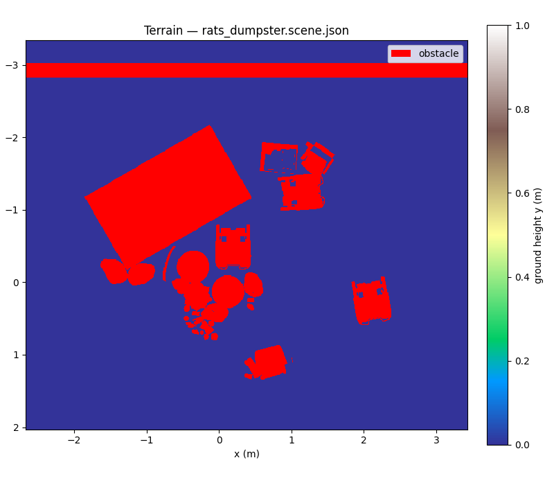
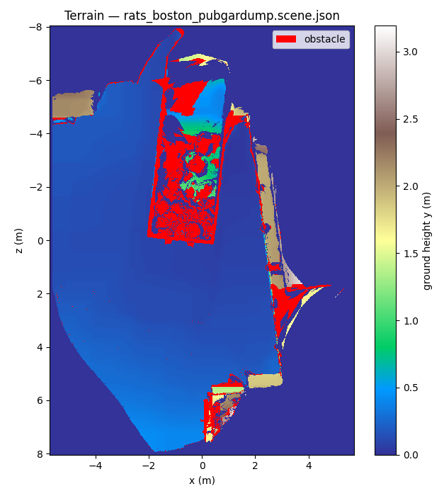
First, we forward predict the particle states z[i,p] with the implemented movement model predict(z[i,p], rng_key). In our particular case, we randomly perturb the 2D velocity on the ground surface and compute the new position with Euler’s method. Again, the height coordinate is inferred automatically based on the exported height maps and movement is constrained by the obstacles automatically inferred with the Blender pipeline. Below we show the height and obstacle maps for the considered scenes.

Second, we have to quantify how well the predicted particle states z[i,p] match the current observations x[j]. For this, we compute the affinity of each tracklet to each observation:

L[i,p,j] = 
  exp(compute_log_likelihood(z[i,p],x[j]))
A[i,j] = sum_p w[i,p] * L[i,p,j]

In our particular case, the likelihood computation predicts the bounding box based on the position and size of the particle state and compares it to the observed bounding box with the intersection over union (IoU) metric.

We add to this matrix the column A[i,M+1] = ghost_prior to model a missed detection—a tracklet is a ghost if we cannot match an observation to it. We also add a row A[T+1,j] = birth_prior to model unexplained detections - an observation that cannot be explained by any active tracklet. In this approach, A[T+1,M+1] = 1 is called the slack cell. To interpret the affinity as probabilities, we want each row and column to sum to 1. We achieve this with a version of Sinkhorn’s algorithm. ¹³ After this normalization, the value of the slack cell can be interpreted as the mass of all successful matches. Note that this data association strategy is inspired by the PDA / JPDA approach. ¹⁴

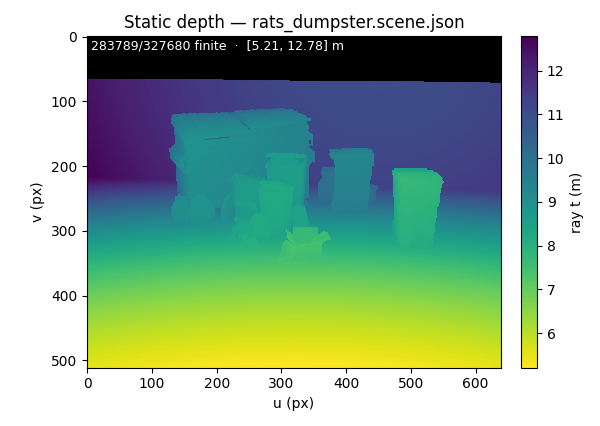
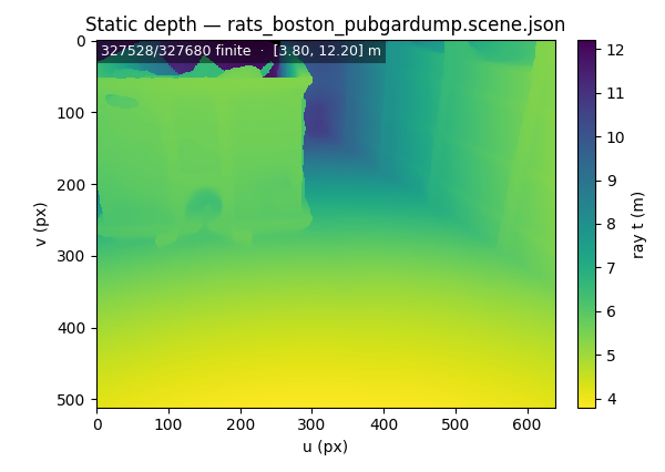
Third, there is another explanation for missing detections: occlusions. If we know where rats may enter or leave the scene and where objects are located in the 3D environment, we can reason about rats being occluded. The particular occlusion logic used in this work is implemented based on the exported depth maps. We can simply compare the depth of an environment object to the distance of a particle position with respect to the same camera ray. If the particle is further away than the object, it has to be occluded. See the depth maps below.

Fourth, we update the particle weights based on the data association and the ghost probability, which is gated by occlusion_miss.

w[i,p] = w[i,p] *
    (data_assoc + ghost * occlusion_miss)

Above, data_assoc = sum_j A[i,j] * L[i,p,j] is proportional to the probability that a particle matches any observation, ghost = A[i,M+1] is the probability that tracklet i is missing an observation, and occlusion_miss = is_occluded(z[i,p]) * (ghost > thresh) allows missing observations (ghosts) to be explained by occlusions.

Fifth, predicted particle states that do not explain the new data well will be assigned a weight close to zero. In a resampling step, we get rid of those particles and duplicate the higher weighted states. A challenging case arises when hypotheses - particle states - become multi-modal. This may happen when, due to noise and overlapping bounding boxes, the algorithm cannot resolve the uncertainty in the data association: two bounding boxes could explain the same rat. Naive resampling collapses multi-modal hypotheses to the strongest mode. Thus, we perform stratified resampling with respect to the data association to keep all plausible modes alive.

Lastly, we keep track of how often an observation cannot be explained by any tracklet and how often a tracklet is a ghost. If these counts exceed some threshold, we spawn a new tracklet or deactivate the ghost tracklet, respectively. Once it is decided to spawn a new tracklet, we allow customization with init_at_observation to initialize high quality particle states for the new observations. For instance, we can take the center of a new bounding box and project it onto the ground surface to get good estimates for the initial position of the newly appeared rat. Furthermore, birth_probability(x[j]) can be used to control the probability that a yet undetected rat appears with the unmatched observation x[j]. For instance, we may increase the probability when bounding boxes are near burrows or the edge of the frame. Likewise, we may set it to 0 on flat surfaces where no undetected rats should suddenly pop up.

Demonstration

To demonstrate the capabilities of our tracking implementation we briefly discuss the results on the dumpster and Boston scenes.

In the first frames of the video, rats appear from their burrows. Since there are no active tracklets that explain these observations, new tracklets are spawned. Shortly after 10 seconds, the paths of tracklets 6 and 7 start to overlap and label uncertainty increases. Note that the association matrix splits the corresponding bounding boxes almost evenly among these tracklets, resulting in multi-modal hypotheses. In the rest of the video, you see rats leaving the frame or disappearing into their burrows. In these cases, they become ghosts and the tracklets are deactivated after a few frames.

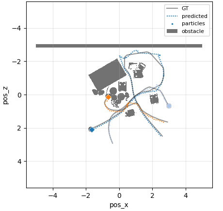
The dumpster scene illustrates the tracker’s behavior under occlusions. When rats disappear behind boxes or trash cans, you can see that the particles begin to spread out in the shadow of these objects. We lose track of the exact position of the rats, but we know which object they are behind. Once they reappear with a new bounding box, the particles immediately snap back. Below you can see a top-down view of the inferred tracks. The tracks are uncertain behind occlusions and do not exactly match the ground truth, which is expected. But importantly, the tracker does not lose the identity of any of the rats as they reappear.

Future work

This blog highlighted some of our recent progress developing methods to quantify wild animal behavior, and described some challenges we are still working to overcome. While we were able to demonstrate the capabilities of our implemented tracking algorithm on synthetic data, it is left for future work to tune the algorithm to handle the noisy observations of real world data. The model may also be further improved: for instance, real 3D movement instead of restriction to a 2D surface, enhanced prediction step to capture erratic movement of rats, or a directed ellipsoid approximation of rats instead of the current sphere approximation.

The work described here is part of a larger research program to understand the social behavior and cognition of urban rats and other animals in their natural habitats. We are motivated by the concept of “Umwelt” (the unique, subjective sensory world that each living organism experiences and inhabits, shaped by the limits of its body and sense organs), popularized in Ed Yong’s book “An Immense World”. In addition to the work described here, we are working on deciphering rat vocalizations, which occur in frequencies beyond human hearing, and on computational tools for inferring animals’ value functions, strategies, and affective states from observing their behavior. We are also partnering with municipalities and other groups leading welfare-aware rat management efforts. We’d love to hear from folks interested in supporting our work, or partnering with us on new applications of these methods.

References

Peterson, R.E., Batenkov, D., El Hady, A. and Mackevicius, E.L., 2025. Computational urban ecology of New York City rats. bioRxiv. https://doi.org/10.1101/2025.07.21.665423. ↩︎ ↩︎
Kerbl, B., Kopanas, G., Leimkühler, T. and Drettakis, G. 3D Gaussian Splatting for Real-Time Radiance Field Rendering. ACM Transactions on Graphics 42(4), 2023. https://doi.org/10.1145/3592433. ↩︎
Wang, J., Chen, M., Karaev, N., Vedaldi, A., Rupprecht, C. and Novotny, D. VGGT: Visual Geometry Grounded Transformer. CVPR 2025. https://arxiv.org/abs/2503.11651. ↩︎
Aitsahalia, I., Botch, T.L., Gu, S., O’Connell, T., Siegel, R., Peterson, R.E., Batenkov, D. and Mackevicius, E.L., Inferring cognitive strategies from groups of animals in natural environments. In NeurIPS 2025 Workshop: Data on the Brain & Mind Findings. https://openreview.net/pdf?id=mUPCoCIxLK. ↩︎ ↩︎ ↩︎
Barsellotti, L., Bianchi, L., Messina, N., Carrara, F., Cornia, M., Baraldi, L., Falchi, F. and Cucchiara, R. Talking to DINO: Bridging Self-Supervised Vision Backbones with Language for Open-Vocabulary Segmentation. ICCV 2025. https://arxiv.org/abs/2411.19331. ↩︎
Plum, F., Bulla, R., Beck, H.K., Imirzian, N. and Labonte, D. replicAnt: a pipeline for generating annotated images of animals in complex environments using Unreal Engine. Nature Communications 14, 7195 (2023). https://doi.org/10.1038/s41467-023-42898-9. ↩︎
Urbaniak, Rafal, Marjorie Xie, and Emily Mackevicius. “Linking cognitive strategy, neural mechanism, and movement statistics in group foraging behaviors.” Scientific Reports 14.1 (2024): 21770. https://doi.org/10.1038/s41598-024-71931-0. ↩︎
Jocher, G., Qiu, J. and Chaurasia, A. Ultralytics YOLO. 2023. https://github.com/ultralytics/ultralytics. ↩︎
Zhang et al. ByteTrack: Multi-Object Tracking by Associating Every Detection Box. ECCV 2022. https://doi.org/10.1007/978-3-031-20047-2_1. ↩︎ ↩︎
Skorokhodov, V., Xu, C., Sun, S., Fink, O. and Mielle, M. SEAR: Simple and Efficient Adaptation of Visual Geometric Transformers for Unpaired RGB-Thermal 3D Reconstruction. arXiv:2603.18774, 2026. https://arxiv.org/abs/2603.18774. ↩︎
Chopin, N. and Papaspiliopoulos, O. An Introduction to Sequential Monte Carlo. Springer Series in Statistics, Springer, 2020. https://doi.org/10.1007/978-3-030-47845-2. ↩︎
Arulampalam et al. A tutorial on particle filters for online nonlinear/non-Gaussian Bayesian tracking. IEEE Trans. Signal Process., 2002. https://doi.org/10.1109/78.978374. ↩︎
Sinkhorn, Richard, & Knopp, Paul. (1967). Concerning nonnegative matrices and doubly stochastic matrices. Pacific J. Math. 21, 343–348. https://dx.doi.org/10.2140/pjm.1967.21.343. ↩︎
Bar-Shalom, Y. and Fortmann, T.E. Tracking and Data Association. Mathematics in Science and Engineering, vol. 179. Academic Press, 1988. ISBN 978-0-12-079760-8. ↩︎