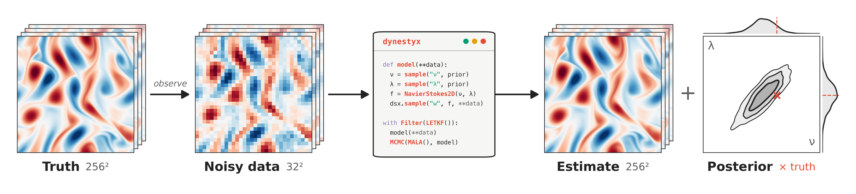
Researchers who study evolving, or “dynamical,” systems—from epidemics to turbulent flows—often need to adapt their models and methods as new data and questions arise. Current software can make this difficult, requiring substantial code to be rewritten. That’s why we developed Dynestyx, a software toolkit that lets researchers build custom dynamical models and access a wide range of state-of-the-art inference methods to learn from real-world data. A shared interface and sensible defaults make it easier to adapt their analysis without rebuilding it each time.
Dynestyx is a probabilistic programming library for dynamical systems.
At Basis, we’re developing a platform of core modeling and reasoning technologies that researchers can build on and use across science and engineering projects. We focus on shared computational needs: a technology created to address a challenge in one field can spur progress in another. Our goal is for this platform to include models verified by experts in formal methods, giving researchers a stronger foundation for analyses they can trust.
A year ago, we set out to build one such technology, dynestyx, to help applied and methodological researchers, scientists, and engineers work with models and data from dynamical systems to answer key questions like:
Forecasting. What will happen next in this system?
State inference. Where has the system been?
System identification. How does the system work, and what are its rules?
Counterfactual inference. What will happen if I intervene on the system?
Good answers to these questions are paired with quantified uncertainty—that is, a measure in how confident we are in our answer. The best answers also address the meta-question: how reliable is the assessment of uncertainty?
We built dynestyx to solve a real gap between practice and theory: that applied researchers often use suboptimal methods to answer these questions, and methodologists commonly develop new methods without real-world challenges in mind. dynestyx1 is a probabilistic programming2 library (like Stan, NumPyro, and PyMC) for dynamical systems that provides a single, clean interface for trying and evaluating different methods and models. Let’s step through a few design principles of dynestyx.
Choosing a method shouldn’t mean rebuilding an analysis
Answering questions about forecasting, inference, system identification, or counterfactuals requires choices: how we represent a system, which inference method we should use, and how to assess the resulting uncertainty. Researchers need to be able to revisit those choices as their data, questions, and methods evolve.
This is a mathematical problem, but too often, software becomes the bottleneck. Methods developed for closely related problems live in separate packages, each with its own model definitions, assumptions, and data interfaces; trying another method can thus mean rebuilding an entire analysis. Applied researchers face a substantial cost when comparing alternatives, while methodological researchers face the same barrier in benchmarking new algorithms on real problems.
We believe researchers should be able to describe a dynamical system once, apply compatible inference methods, and examine how those choices affect their conclusions. A shared foundation would make methodological advances easier to use—and practical challenges easier to bring back into methodological research. It also makes it easier to use the best method available under a given set of assumptions, and to determine empirically what that best method actually is.
We should work within an ecosystem
dynestyx gains much of its flexibility and power by leveraging already rich JAX scientific computing libraries. This creates a reinforcing ecosystem, allowing more trusted, hardened features, while improving existing libraries as a healthy ecosystem.
As a primary example, dynestyx is built to be fully compatible with NumPyro3 programs. This allows for a rich probabilistic programming syntax, and reliable, optimized approximate Bayesian inference algorithms. We additionally support advanced Monte Carlo algorithms in BlackJAX,4 and a wide array of state-space inference algorithms via cuthbert,5CD-Dynamax,6 and Dynamax.7
dynestyx integrates—and improves on—these existing packages by unifying their disparate pieces into a single interface with sensible defaults. Researchers can change their models, explore the state-of-the-art in methods, and develop new algorithms without rebuilding the surrounding analysis.
Domain scientists can build and share analyses with little implementation work. Method developers can use those same models and workflows to test, compare, and improve algorithms on real problems.
What makes dynestyx so easy to use?
You describe the dynamical system once, then choose how to simulate it, learn from data, and assess the results. Eight features make this practical:
A unified DynamicalModel class. A DynamicalModel brings together an initial_condition for $x_0 \in \mathbb{R}^{d_x}$, a state_evolution describing how the state $x_t \in \mathbb{R}^{d_x}$ changes, and an observation_model relating measurements $y_t \in \mathbb{R}^{d_y}$ to that state. Each component can be random or deterministic, and evolution can be defined in continuous or discrete time—with scope to support hybrids in the future.
Hierarchical models without the bookkeeping.dsx.plate lets you define multiple, related dynamical systems with shared parameters and individual variation, much as NumPyro’s plates support hierarchical Bayesian models. You can pool information across experiments, individuals, or trajectories while allowing each system to behave differently.
Compose the task you want to perform. Handlers specify how to combine a model with data: dsx.Filter and dsx.Smoother estimate hidden states; dsx.LatentPathBuilder exposes state paths for inference; dsx.Discretizer controls how continuous dynamics are discretized; dsx.Simulator generates trajectories; and dsx.Evaluation scores predictions. These components fit together around the same model definition.
NumPyro inference when you want it.dynestyx models work with NumPyro’s existing parameter-inference machinery, including the No-U-Turn Sampler (NUTS) and stochastic variational inference (SVI). You can also use dynestyx directly for simulation, state estimation, and optimization without ever writing a NumPyro program.
Swap algorithms with minimal changes. Filters, solvers, samplers, and their settings are configurable. For compatible models, switching from a differentiable particle filter inside NUTS to an autodifferentiable ensemble Kalman filter (EnKF) with SVI can take just two lines: change the filter configuration and the parameter-inference method.
Sensible defaults, with the choices explained. Omit the handlers and dynestyx identifies the task from your model and inputs, selects compatible inference and numerical methods, and reports its choices. You can inspect the decisions and override them as needed.
Missing data handled where it belongs. Measurements may arrive at different times, individual sensors may go silent, or entire observations may be missing. Mark unavailable entries with NaN; dynestyx uses statistical treatments suited to the observation model, such as marginalizing unobserved components of Gaussian measurements.
Evaluation alongside inference. A shared evaluation and diagnostics platform helps you assess prediction quality and uncertainty, compare algorithms on the same data, and judge how much to trust a particular model and numerical implementation.
dynestyx makes human–AI collaboration easier. Its clear interfaces and composable numerical components help AI write shorter, better code that researchers can read, verify, understand, and refine.
Example Gallery
SDEs in Dynestyx
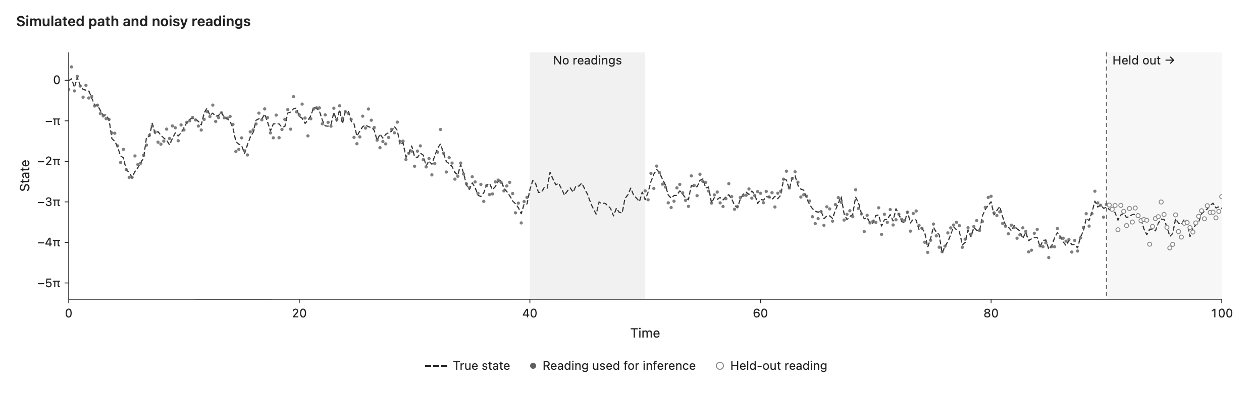
SDEs are easy to implement in dynestyx! In this example, we are going to model a particle starting at $X_0 \sim \mathcal{N}(0, 1)$, and evolving over time according to the SDE $\mathrm{d}X_t = \alpha \sin(X_t) \, \mathrm{d}t + \mathrm{d}W_t$, where $\alpha$ is an unknown parameter with prior $\alpha \sim \textrm{HalfNormal}(0.5)$. This SDE “pulls” towards equilibria at $(2k+1)\pi$, with the force of that pull controlled by $\alpha$. We obtain measurements for $0 \leq t \leq 100$ embedded in Gaussian noise; our goal is to infer $\alpha$, and make filtering and forecasting predictions accordingly.
The underlying generated state is shown in the dashed line, and dots are noisy measurements. Solid dots are observed, and hollow dots are held out.
dynestyx offers many ways to perform parameter inference. Here, we compare the particle filter with adaptive Metropolis (a form of particle MCMC; Andrieu et al., 2010), the EnKF with NUTS, and the EnKF with stochastic variational inference.
Using learned parameters, we can perform both filtering and forecasting with robust uncertainty quantification. We show filtering in green, including a period with missing observations, and forecasting using the EnKF + NUTS posterior.
Inside the example
Excerpts from the executed example.
defmodel(obs_times=None,obs_values=None,ctrl_times=None,ctrl_values=None,predict_times=None):# Sample one positive drift rate for this path.alpha=numpyro.sample("alpha",dist.HalfNormal(.5))dynamics=dsx.DynamicalModel(initial_condition=dist.MultivariateNormal(jnp.zeros(1),jnp.eye(1)),state_evolution=dsx.ContinuousTimeStateEvolution(drift=lambdax,u,t:alpha*jnp.sin(x),diffusion=dsx.ScalarDiffusion(1.,bm_dim=1),),observation_model=dsx.LinearGaussianObservation(H=jnp.eye(1),R=0.5**2*jnp.eye(1)),)returndsx.sample("x",dynamics,obs_times=obs_times,obs_values=obs_values,predict_times=predict_times)# Simulate a latent path and noisy observations.t=jnp.linspace(0.,100.,401)withdsx.Simulator():sim=Predictive(model,num_samples=1)(jr.PRNGKey(7),predict_times=t)
# Fit only readings through t = 90; leave later observations for validation.t=jnp.linspace(0.,100.,401)seen=t<=90obs_times=t[seen]# The sensor is silent for 40 <= t < 50: mark those readings as missing.gap=(t>=40)&(t<50)obs_values=jnp.where(gap[:,None],jnp.nan,sim["x_observations"][0,0])[seen]# Fitting needs only the likelihood, so skip saving filter outputs per draw.quiet=dict(record_filtered_particles=False,record_filtered_log_weights=False,record_filtered_states_mean=False,record_filtered_states_cov=False,record_filtered_states_cov_diag=False,include_predicted_observations=False)# PF + AdaptiveMetropolis: this filter takes only the observed times.keep=~jnp.isnan(obs_values[:,0])withdsx.Filter(PFConfig(n_particles=512,**quiet)):withdsx.Discretizer(EulerMaruyamaConfig()):config=AdaptiveMetropolisConfig(num_samples=4000,num_warmup=2000,num_chains=4)fit=MCMCInference(config,model)draws=fit.run(jr.PRNGKey(3),obs_times[keep],obs_values[keep])# EnKF + NUTS: four chains of 1,000 warmup and 1,000 kept drawswithdsx.Filter(EnKFConfig(n_particles=64,**quiet)):withdsx.Discretizer(EulerMaruyamaConfig()):fit=MCMC(NUTS(model,init_strategy=init_to_median,max_tree_depth=5),num_warmup=1000,num_samples=1000,num_chains=4,chain_method="sequential",progress_bar=False)fit.run(jr.PRNGKey(2),obs_times=obs_times,obs_values=obs_values)nuts_draws=fit.get_samples()# EnKF + SVI (multivariate-normal guide)withdsx.Filter(EnKFConfig(n_particles=64,**quiet)):withdsx.Discretizer(EulerMaruyamaConfig()):guide=AutoMultivariateNormal(model,init_loc_fn=init_to_median,init_scale=.5)fit=SVI(model,guide,numpyro.optim.Adam(.003),Trace_ELBO(num_particles=8))result=fit.run(jr.PRNGKey(4),8000,obs_times=obs_times,obs_values=obs_values)draws=guide.sample_posterior(jr.PRNGKey(5),result.params,sample_shape=(4000,))
# Keep 200 of the 4,000 NUTS draws from the fit to readings through t = 90.draws={"alpha":nuts_draws["alpha"][::20]}pred=Predictive(model,posterior_samples=draws,parallel=True,condition_deterministic=False)# Predict from t = 0 to 100, conditioning only on readings through t = 90.t=jnp.linspace(0.,100.,401)withdsx.Simulator(n_simulations=8):withdsx.Filter(EnKFConfig(n_particles=64)):withdsx.Discretizer(EulerMaruyamaConfig()):result=pred(jr.PRNGKey(6),obs_times=obs_times,obs_values=obs_values,predict_times=t)# Summarize across both parameter draws and stochastic rollouts.paths=result["x_predicted_states"][...,0]# Median with 50%, 80%, and 95% bands.bands=jnp.quantile(paths,jnp.array([.025,.1,.25,.5,.75,.9,.975]),axis=(0,1))
Hierarchical SDEs in Dynestyx
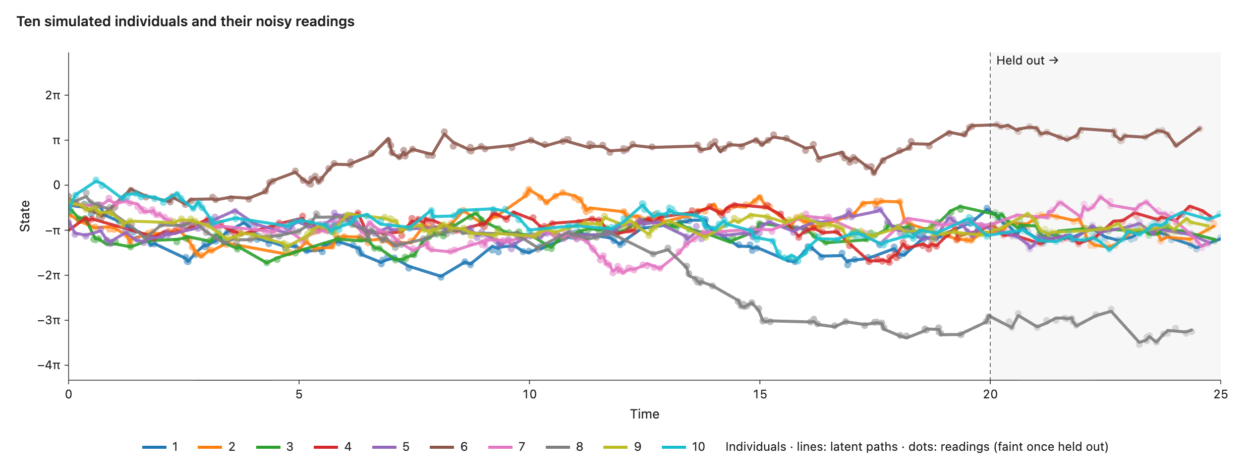
Many processes in the sciences entail the dynamics of many individuals, each unique but related. dynestyx makes it easy to model such processes (which we call “hierarchical SSMs”) using a “plate” construct. In this case, we illustrate simulation, system identification, and filtering & forecasting on a hierarchical version of the sinusoidal well SDE; each individual draws $\log\alpha_i \sim \mathcal{N}(\mu_g, \sigma^2)$, initial means follow $m_i \sim \mathcal{N}(m_g, \sigma_0^2)$, and initial conditions are set as $X_{i0} \sim \mathcal{N}(m_i, 0.05^2)$. We set global priors for $\mu_g, \sigma, m_g, \sigma_0$, and perform Bayesian inference on individual and global parameters. This process is compatible with multiple levels of hierarchy, as well!
We simulate ten individuals, each with their own color. Lines are the latent paths, and dots are their noisy measurements. Readings after t = 20 are held out for forecasting.
Left: the four population parameters, and their estimated posteriors with EnKF + NUTS. Center and right: each individual’s drift rate and initial mean, respectively, and its Bayesian posterior.
The filtered and forecasted estimates of each individual, using the posterior parameter estimates of EnKF + NUTS.
Inside the example
Excerpts from the executed example.
classSineDrift(eqx.Module):alpha:jax.Arraydef__call__(self,x,u,t):returnself.alpha*jnp.sin(x)defmodel(obs_times=None,obs_values=None,predict_times=None):# Draw the centers and spreads of the two populations.mu_g=numpyro.sample("mu_g",dist.Normal(0.,.5))sigma=numpyro.sample("sigma",dist.HalfNormal(.5))m_g=numpyro.sample("m_g",dist.Normal(0.,2.))sigma0=numpyro.sample("sigma0",dist.HalfNormal(2.))withdsx.plate("individuals",10):# Noncentered effects give each individual a rate and starting mean.z=numpyro.sample("z",dist.Normal(0.,1.))z0=numpyro.sample("z0",dist.Normal(0.,1.))alpha=jnp.exp(mu_g+sigma*z)m=m_g+sigma0*z0dynamics=dsx.DynamicalModel(initial_condition=dist.MultivariateNormal(m[...,None],.05**2*jnp.eye(1)),state_evolution=dsx.ContinuousTimeStateEvolution(drift=SineDrift(alpha),diffusion=dsx.ScalarDiffusion(1.,bm_dim=1),),observation_model=dsx.LinearGaussianObservation(H=jnp.eye(1),R=0.1**2*jnp.eye(1)),)returndsx.sample("x",dynamics,obs_times=obs_times,obs_values=obs_values,predict_times=predict_times)# Read each individual at its own random times: t = 0, then 99 times# before t = 20 and 25 held-out times after it.rng=np.random.default_rng(11)times=jnp.asarray(np.stack([np.r_[0.,np.sort(rng.uniform(0.,20.,99)),np.sort(rng.uniform(20.,25.,25))]for_inrange(10)]))# Simulate latent paths and noisy readings at those times.withdsx.Simulator():sim=Predictive(model,num_samples=1)(jr.PRNGKey(7),predict_times=times)
# Fit each individual's 100 readings before t = 20; hold out the rest.# Euler-Maruyama takes one step per interval, so add unobserved times# every 0.05 (NaN readings, which the EnKF skips) to keep steps short.grid=np.arange(.05,20.,.05)obs_times,obs_values=[],[]fort,yinzip(np.asarray(times[:,:100]),np.asarray(sim["x_observations"][0,:,0,:100,0])):g=grid[np.min(np.abs(grid[:,None]-t[None,:]),axis=1)>.01]order=np.argsort(np.r_[t,g])obs_times.append(np.r_[t,g][order])obs_values.append(np.r_[y,np.full(len(g),np.nan)][order])# (Each individual is then padded to a common length with midpoints of its widest gaps.)obs_times,obs_values=jnp.asarray(np.stack(obs_times)),jnp.asarray(np.stack(obs_values))[...,None]# Fitting needs only the likelihood, so skip saving filter outputs per draw.quiet=dict(record_filtered_particles=False,record_filtered_log_weights=False,record_filtered_states_mean=False,record_filtered_states_cov=False,record_filtered_states_cov_diag=False,include_predicted_observations=False)# EnKF + NUTS: four chains of 500 warmup and 500 kept draws, run in parallel# (after numpyro.set_host_device_count(4)).withdsx.Filter(EnKFConfig(n_particles=32,**quiet)):withdsx.Discretizer(EulerMaruyamaConfig()):fit=MCMC(NUTS(model,init_strategy=init_to_median,max_tree_depth=5),num_warmup=500,num_samples=500,num_chains=4,chain_method="parallel",progress_bar=False)fit.run(jr.PRNGKey(2),obs_times=obs_times,obs_values=obs_values)nuts_draws=fit.get_samples()# Recover individual drift rates and starting means in each posterior draw.alpha=jnp.exp(nuts_draws["mu_g"][:,None]+nuts_draws["sigma"][:,None]*nuts_draws["z"])m=nuts_draws["m_g"][:,None]+nuts_draws["sigma0"][:,None]*nuts_draws["z0"]
# Keep 200 of the 2,000 NUTS draws from the fit to readings before t = 20.keys=("mu_g","sigma","m_g","sigma0","z","z0")draws={k:nuts_draws[k][::10]forkinkeys}pred=Predictive(model,posterior_samples=draws,parallel=True,condition_deterministic=False)# Predict on a regular grid from t = 0 to 25, conditioning only on readings before t = 20.grid=jnp.linspace(0.,25.,201)withdsx.Simulator(n_simulations=8):withdsx.Filter(EnKFConfig(n_particles=32)):withdsx.Discretizer(EulerMaruyamaConfig()):result=pred(jr.PRNGKey(6),obs_times=obs_times,obs_values=obs_values,predict_times=grid)# Summarize across both parameter draws and stochastic rollouts.paths=result["x_predicted_states"][...,0]# Median with 50%, 80%, and 95% bands.bands=jnp.quantile(paths,jnp.array([.025,.1,.25,.5,.75,.9,.975]),axis=(0,2))
Navier Stokes
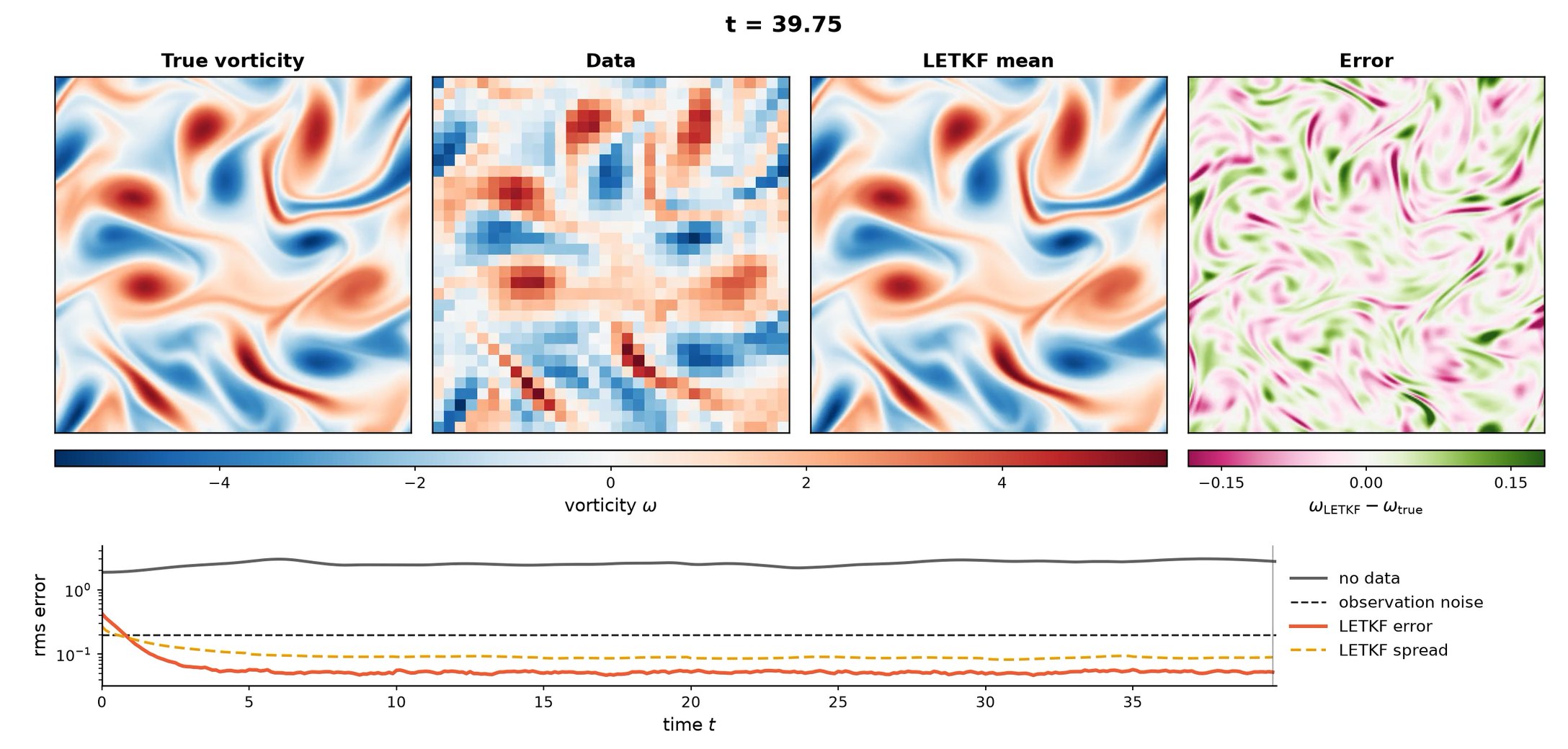
dynestyx also allows us to model PDEs that are parameterized on a constant-dimensional state, and even perform parameter estimates therein! Here, we illustrate this with fluids simulated according to a Navier Stokes flow. This includes filtering on a 256×256-dimensional posterior, parameter estimation over a smaller grid, and closed-loop control of particles in a fluid.
Using a local ensemble Kalman filter (LETKF; Hunt et al., 2007), we can estimate a true, high-resolution (256×256) flow (left) using low-dimensional (32×32) and noisy observations (center-left), visualizing the filtered mean (center-right) and its error (right). We show its RMS relative to the noise scale (bottom). The flow is described by the Navier Stokes equations with Kolmogorov forcing, generated by integrating exponax (Koehler et al., 2024) into dynestyx.
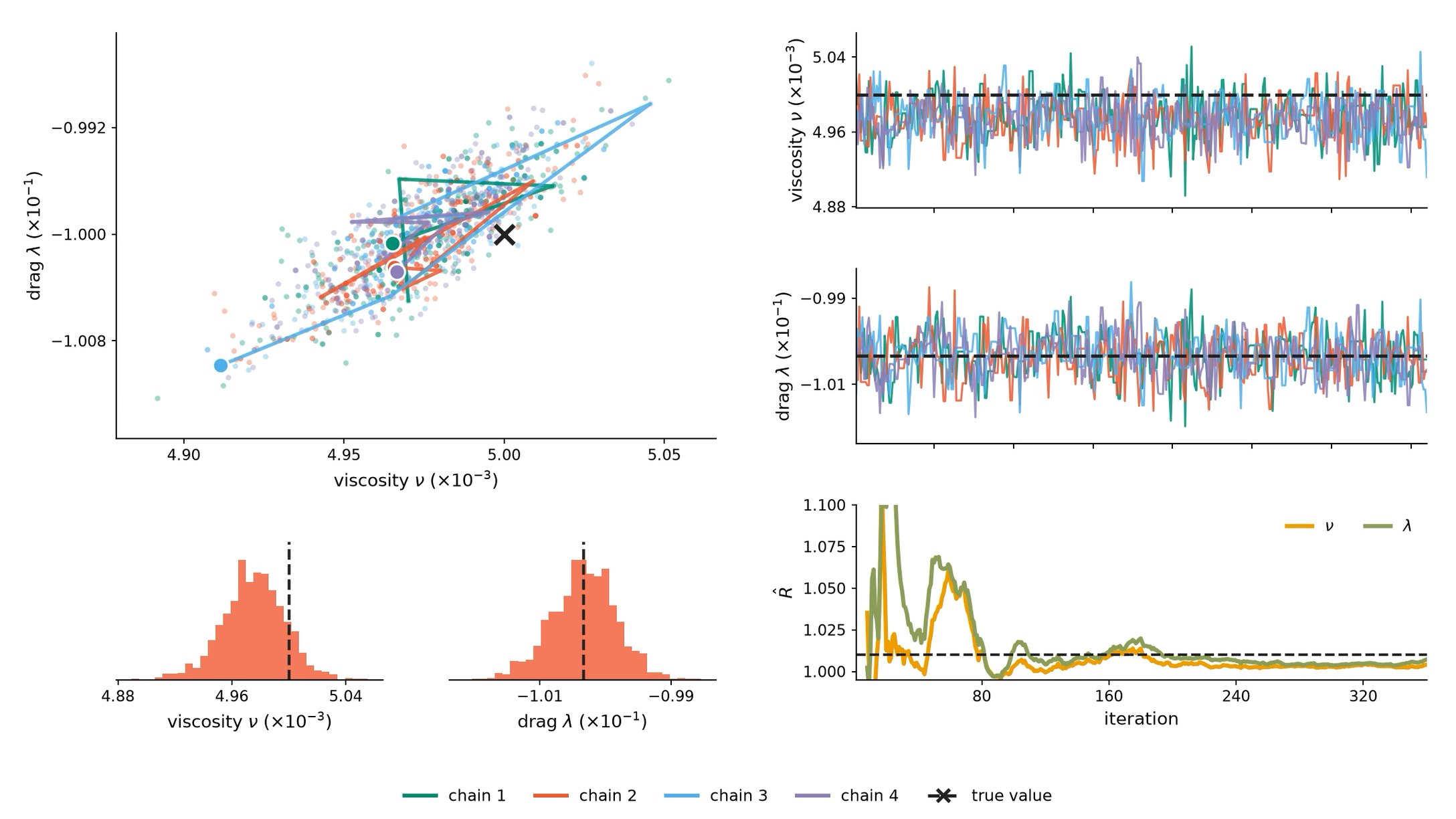
From data, we can estimate, with uncertainty, the values of parameters of the flow. For example, by running MALA on data from a 16×16×16 simulation of the Navier Stokes equations with Kolmogorov forcing, we obtain well-mixing estimates of viscosity and drag covering the truth.
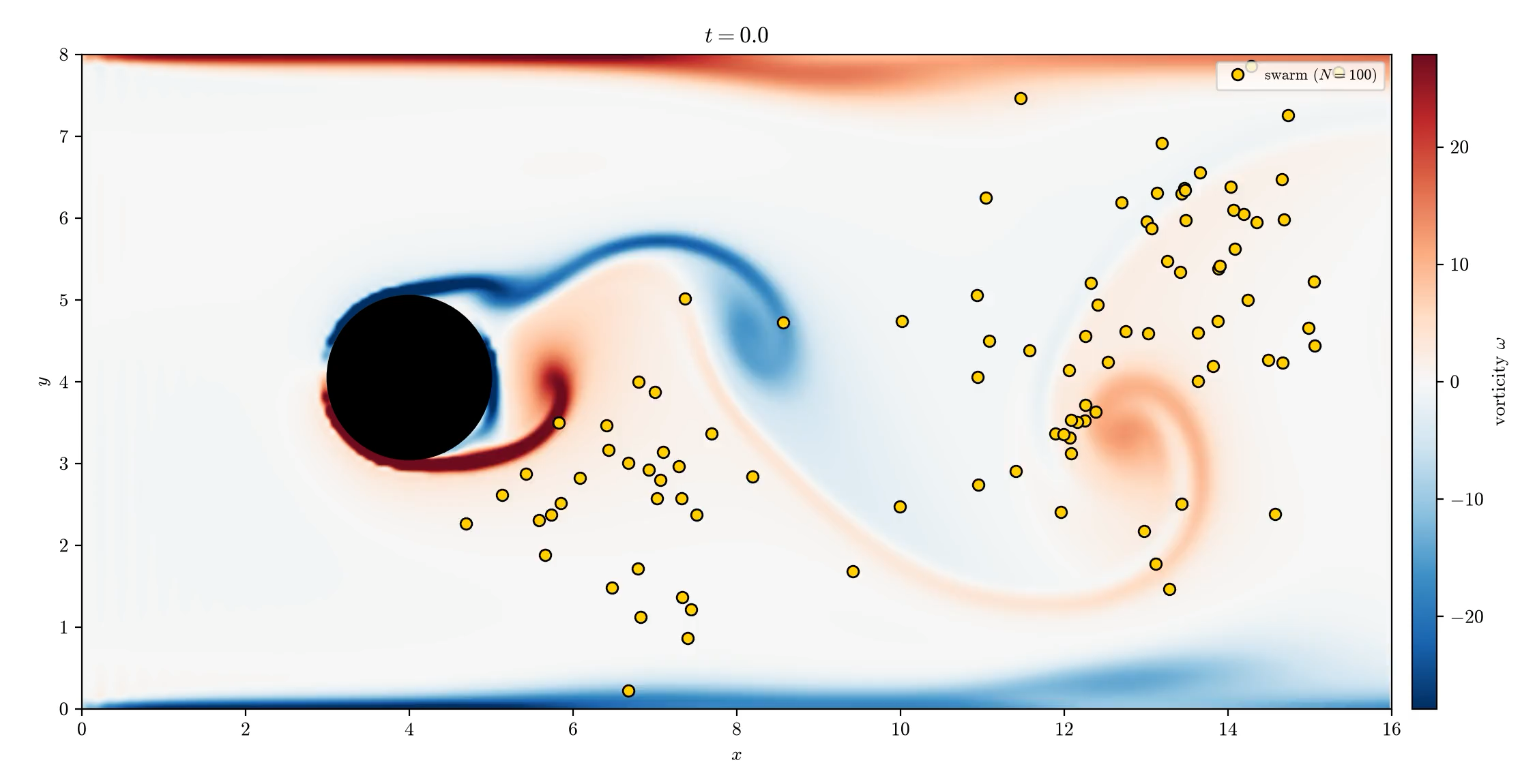
dynestyx allows us to compose PDE simulation with closed-loop control; in this example, we simulate fluid flow around a cylinder, and control a set of particles using a “swarm” policy (PI control + a repulsive term) to approach the right edge of the cylinder. In this case, we use PhiFlow (Holl et al., 2020) for fluid simulation.
Robotic manipulation
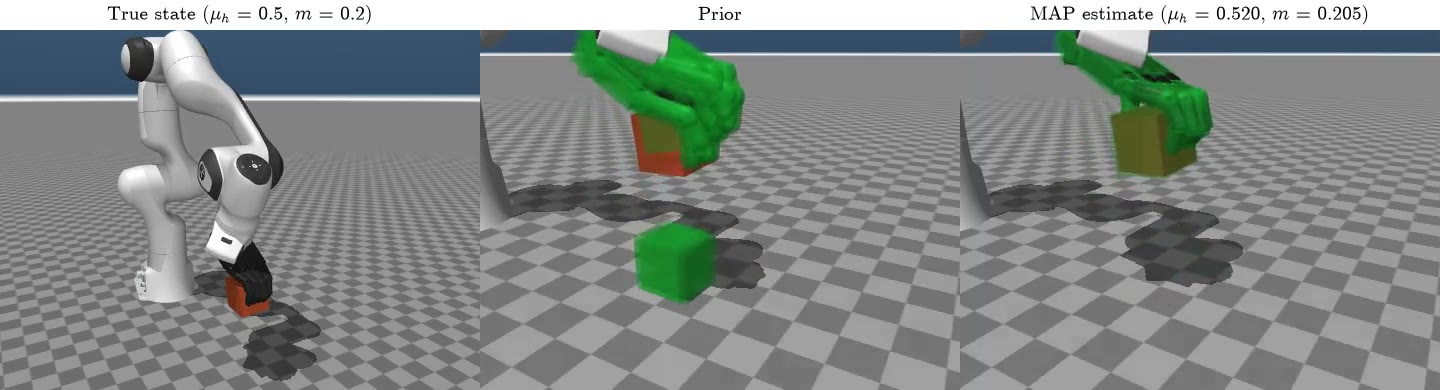
A robot’s grasp depends on physical properties it may not know in
advance: how heavy an object is and how much friction its fingers
provide. Here, we use dynestyx to infer those properties from a simulated
grasp, fitting a MuJoCo model to the reference motion and then replaying
the lift with the learned mass and friction.
Robots in the real world also rarely get to read off the exact state of
the objects they handle; they have to act on what their sensors suggest.
In a second example, a robot hand moves a cube into a desired orientation.
The position and velocity of the cube are unknown and must be inferred
from camera images. A Kalman filter integrates the camera images into an
estimate of the cube’s state, and a model-predictive controller plans
ahead from that state.
The left panel is the reference grasp. The middle overlays motions simulated before the mass and friction are learned; cubes can slip, fall, or follow different paths. The right shows the motion after dynestyx fits those properties. Compare the fitted motion with the reference to see how learning the physical properties improves the simulation.
The left panel shows the true trajectory of the cube. The right panel shows a superposition of some probable cube trajectories, drawn from the filter estimate. Control is the same in both panels, found based on the uncertain belief on the right. The floating cube in the background is the target orientation.
Neural SDE agent tracking
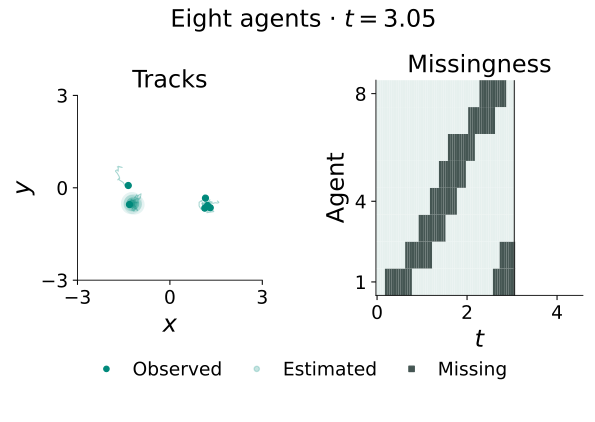
Tracking moving objects becomes difficult when a sensor loses sight of them. Here, we use dynestyx to track eight simulated agents as their position measurements disappear and return, using a fixed landscape model learned from earlier recordings. This shows how learned dynamics can support position estimates and quantify uncertainty during gaps in the data.
The left plot shows agent positions and trails. Black dots are measurements; teal dots and trails show estimated motion. Pale teal marks indicate agents that are currently unobserved, and shaded regions show positional uncertainty. The chart on the right shows which agents have measurements at each time. Watch the estimates spread out during gaps and tighten when observations return.
The two colored maps compare the landscape that generated the agents’ motion (left) with the landscape learned from earlier recordings (right). Both use the same color scale. The white outline marks the region covered by training data. Watch where the moving agents sit relative to the landscape’s wells.
Learning and forecasting an epidemic day by day
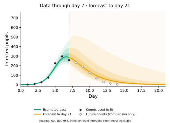
During an outbreak, public-health teams need to estimate how fast infections spread and what may happen next from limited illness counts. Here, we use dynestyx to fit a susceptible–infected–recovered (SIR) model to daily counts from the 1978 English boarding-school influenza outbreak.8 Each day, we refit the model using all counts observed so far, updating estimates of transmission, recovery, and observation noise along with their uncertainty. Those updated parameter distributions drive a new forecast through day 21.
Solid dark dots are counts already used to fit the model; hollow gray circles are future counts shown only for comparison. The dotted line separates the observed past from the forecast, which always extends to day 21. Teal shows the estimated past and orange shows the forecast. The bands contain 50%, 80%, and 95% of plausible underlying infection levels; they exclude day-to-day count noise. Move the slider to see how the forecast and its uncertainty change as more counts become available.
Each day’s curves come from a fresh fit to all counts observed so far. They show what the data suggest about disease spread, recovery, measurement variability, and how many people each infection may generate. Gray dashed curves show the starting assumptions; teal curves show the updated estimates. Narrower curves indicate more precise estimates.
This plot compares one- to seven-day forecasts from the epidemic model with two simpler approaches: carrying the latest count forward and learning a simple relationship between consecutive days. Lower scores mean predictions that better match subsequently observed counts. Each forecast is scored only once the day it predicted has arrived.
Equation discovery for neural circuits
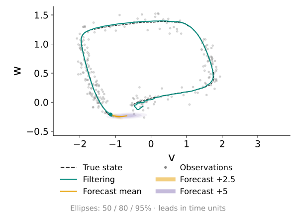
Noisy recordings may reveal a system’s repeated cycles without telling us which equations drive them. Here, we use dynestyx to discover compact equations for a simulated neural model with two interacting quantities. We use Bayesian inference to identify important terms from a larger library, then test the learned dynamics on a new recording by tracking and forecasting through gaps in the observations. The Bayesian formulation accounts for missing observations and stochastic dynamics directly, where many regression-based equation-discovery methods need additional preprocessing or extensions.
The loop on the left shows how the two quantities, v and w, move together; the plots on the right show each one over time. Gray dots are noisy measurements and dashed black lines show the simulated truth. Teal follows the estimated motion, orange shows a forecast, and shaded regions show uncertainty about the estimated and future motion.
Each row is a candidate term in an equation. Teal marks and bars show its estimated strength and uncertainty; diamonds mark the values used to simulate the system. Terms concentrated near zero contribute little to the dynamics. Compare the two panels to see the equations learned for v and w.
Learning to track forty interacting variables
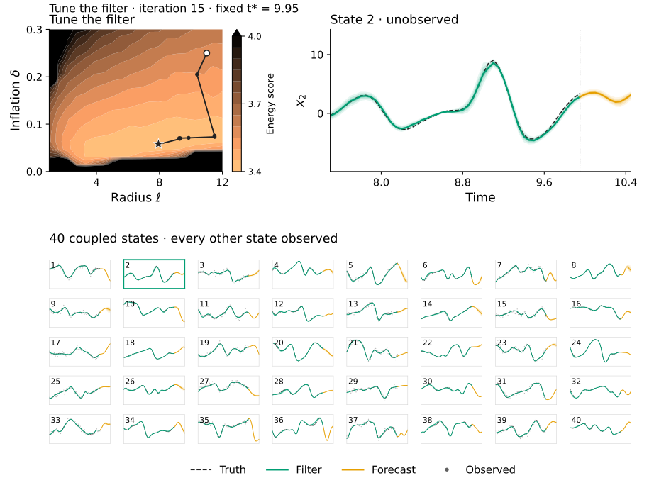
In large systems, observing every variable may be impossible, and a tracking method’s settings can strongly affect its predictions. Here, we use dynestyx to tune a filter (fitting the so-called “localization parameters”) for Lorenz–96, a chaotic model with 40 interacting variables, only half of which we observe. We learn two filter settings from one time window, then hold them fixed while tracking and forecasting all 40 variables in another.
The map compares prediction quality across two settings: how far information is shared between variables (horizontal axis) and how much the method expands its uncertainty estimates (vertical axis). Lighter colors mean better predictions; the path shows tuning progress. The time plots update using the same observations throughout, so changes reflect the new settings. Select a small plot to inspect a variable above.
The large time plot follows the selected variable, while the small plots show all 40. Gray dots mark measurements; variables without dots are inferred through their interactions with the others. Teal is the current estimate, orange is a short forecast, and shaded bands show uncertainty. Dashed black lines show the simulated truth for comparison.
What’s up next?
1. Share some exciting discoveries
Exploring combinations of standard algorithms in dynestyx led us to what we believe is a new best-in-class inference method. It substantially outperformed the alternatives we tested on many of our internal benchmarks. Table 1 of our preprint maps the compositional space; we’ll present the method and results in an upcoming preprint.
2. A comprehensive Bayesian workflow
We are developing a recommended workflow for iteratively refining dynamical models and their inference methods, specializing the Bayesian Workflow9 to the case of dynamics. It will bring together automatic method selection, novel convergence and numerical stability checks, and evaluation of predictions and uncertainty coverage on held-out observations.
We plan to select methods suited to the model and use case: Kalman filtering for linear Gaussian systems, ensemble Kalman filtering for nonlinear systems that pass checks supporting a Gaussian approximation, and no filtering by default when the state is fully observed with high fidelity and frequency. Researchers will be able to inspect and override these choices, using diagnostics to guide further refinement.
3. Next-gen trustworthiness in scientific software
We plan to build formal verification into Basis’s core-technology platform, pairing scientific testing with mathematical guarantees about the code researchers and AI agents actually run. Using proof assistants such as Lean, we will connect proofs to numerical implementations and make assumptions about precision and algorithm settings explicit. We also aim to preserve those guarantees when components are combined, so that trust in individual routines extends to the larger scientific programs built from them.